Posts Tagged ‘electronic energy’

How does one describe the wavefunction for the π-complex formed from PhNHOPh?

Friday, January 25th, 2013

Although have dealt with the π-complex formed by protonation of PhNHOPh in several posts, there was one aspect that I had not really answered; what is the most appropriate description of its electronic nature? Here I do not so much provide an answer, as try to show how difficult getting an accurate answer might be.

pi-complex

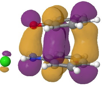
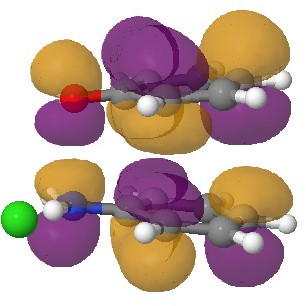
In an earlier post, I had shown how an in-phase combination of the HOMO of the anion 1 with the LUMO of the cation 2 led to an occupied molecular orbital for the complex (below, left). An out-of-phase combination of these two gives instead the LUMO of the π-complex (below, right). It might seem as if a pair of electrons would like to occupy the first of these, and indeed a wavefunction constructed on this basis (using this occupancy as the single reference; indeed only state) resulted in the conclusion that the complex was aromatic. The diatropicity (~magnetic aromaticity) was strongest in the region between the two stacked rings, and the individual rings themselves had lost their local aromaticity. One might then infer that a wavefunction constructed by populating the LUMO below would in fact rearrange the aromaticity, returning this property back to the two individual rings. There would in fact be apparently nothing to keep the rings stacked, and so in the limit this wavefunction would correspond to a biradical (both states would be degenerate and hence have one electron in each). 

The HOMO. Click for  3D.

The π-complex HOMO. Click for 3D.

LUMO. Click for 3D

The π-complex LUMO. Click for 3D

So where along this spectrum of possible interpretations does a more realistic wavefunction settle? To answer this question, we must optimise the self-consistent field describing the electronic structure using BOTH electronic configurations (as a first approximation). This method is known as a multi-reference configuration interaction or CASSCF (complete active space self-consistent field) approach. Technically, the variation principle of minimising the electronic energy is applied to all the eigenvalues of the CI matrix, and not just the single reference state as is normally done. The simplest approach to the molecule above is to consider the active space as just the two orbitals above (the inactive space is represented by all the remaining doubly occupied and unoccupied orbitals), resulting in a CI determinant with three solutions (two electrons in the HOMO, two electrons on the LUMO and one electron in each). One would then use the energy computed from this multi-reference solution to re-optimise the geometry of the π-complex. This would then surely be a “better” description of the wavefunction for this molecule. Or would it? Well, this is what happened when I tried.

  1. I took the geometry previously found for the π-complex (it is pertinent that this was obtained using a density functional method with inclusion of dispersion attractions; ωB97XD/6-311(d,p)/SCRF=water) and ran a CASSCF(2,2) calculation at that geometry (and retaining the solvent field). This means an active space of two orbitals (the two shown above) populated with two electrons in three different configurations. The answer came out that the lowest energy solution (eigenvalue) of the CI matrix had eigenvectors corresponding to 0.94 (two electrons in the HOMO) and -0.34 (two electrons in the LUMO). This translates to an electronic population of 1.77 electrons in the former and 0.23 electrons in the latter. So this molecule shows some noticeable multi-reference character. In that it resembles for example, ozone. Such molecules are often described as awkward, since the simple molecular orbital picture which we use when thinking about doubly occupied orbitals is clearly only an approximation (in this case 1.77 rather than 2.0). We often sweep this thought under the carpet.
  2. I then tried to optimise the geometry of the complex using this new, improved electronic description. Well, slowly, the two rings drifted apart. Very slowly! Remember we have a complex hybrid method operating here; CASSCF(2,2)/6-311G(d,p) under the influence of a continuum solvent field for water (which appears necessary to attempt to describe the nature of two ion-pairs stacking on top of each other). The CI vectors crept towards 0.75 (HOMO) and -0.67 (LUMO), corresponding to electron occupancies of 1.11 and 0.89 (almost equal, i.e. a biradical) and close to the other extreme noted above. During this process, the energy dropped by about 10 kcal/mol. So is this a more realistic solution? 
  3. Well, we have to return to the difference between a density functional method with dispersion correction and CASSCF. The former attempts to allow for dynamic electron correlation, and this is particularly important for stacked π-rings. Getting the correct ring separation distance can only be achieved when such electron correlation is included; it is notably not obtained if a simple Hartree-Fock approach is used. CASSCF is a Hartree-Fock based method that captures the static electron correlation, but NOT that dynamic one.
  4. So this leads us to the next refinement, including CASSCF for static correlation and e.g. a method such as MP2 (CASPT2) to recover some dynamic correlation (and the dispersion attractions). This is tough for a molecule with 75 degrees of (geometrical) freedom, since one really needs analytical first derivatives of the energy to optimise the geometry. This combination (CASSCF, MP2, SCRF=water, analytical first derivatives) is not often found! And one I have not yet attempted to use.

What I did learn is that the balance between a mostly single-reference description of the wavefunction (occupancy of 2.0 in the HOMO above) and a multi-reference description (occupancy of 1.0 in the HOMO, 1.0 in the LUMO) is a fine one, and that balance can be perturbed by other effects, such as how one describes the correlation promoting π-stacking of the rings. And to be fair, I have not yet even found out if a CASSCF(2,2) is good enough. Perhaps it should be CASSCF(10,10), since we do have (at least) ten electrons that could populate our active space? 

Of course, there are many solutions to the above problem (and some might even solve the analytical first derivatives limitation noted above). So if any reader of this blog has knowledge/expertise of this type of calculation, it would be wonderful to know what the answer is for protonated PhNHOPh. It is such an innocent molecule, and yet it seems such a challenge to properly compute its geometry (and aromaticity). 

The weirdest bond of all? Laplacian isosurfaces for [1.1.1]Propellane.

Wednesday, July 21st, 2010

In this post, I will take a look at what must be the most extraordinary small molecule ever made (especially given that it is merely a hydrocarbon). Its peculiarity is the region indicated by the dashed line below. Is it a bond? If so, what kind, given that it would exist sandwiched between two inverted carbon atoms?

1.1.1 Propellane

One (of the many) methods which can be used to characterize bonds is the QTAIM procedure. This identifies the coordinates of stationary points in the electron density ρ(r) (at which point ∇ρ(r) = 0) and characterises them by the properties of the density Hessian at this point. At the coordinate of a so-called bond critical point or BCP, the density Hessian has two negative eigenvalues and one positive one. The sum, or trace of the eigenvalues of the density Hessian at this point, denoted as ∇2ρ(r), provides in this model a characteristic indicator of the type of bond, according to the following qualitative partitions:

  1. ρ(r) > 0, ∇2ρ(r) < 0; covalent
  2. ρ(r) ~0, ∇2ρ(r) > 0; ionic
  3. ρ(r) > 0, ∇2ρ(r) > 0; charge shift

The third category of bond was first characterised by Shaik, Hiberty and co. using valence-bond theory1 and they went on to propose [1.1.1] propellane (above, along with F2) as an exemplar of this type.2 Matching the conclusions drawn from VB theory was the value of the Laplacian. As defined above, for the central C-C bond, both ρ(r) and  ∇2ρ(r) have been calculated to be positive, supporting the identification of this interaction as having charge-shift character.3

The Laplacian represents one of those properties where quantum mechanics meets experiment, in that its value (and that of ρ(r) itself) can be measured by (accurate) X-ray techniques.4 This was recently accomplished for propellane,5 with the same conclusion that the Laplacian in the central C-C region has the significantly positive value of +0.42 au. The electron density ρ(r) at this point was measured as 0.194 au. Calculations5 at the B3LYP/6-311G(d,p) level report ρ(r) as ~0.19 and ∇2ρ(r) as +0.08 au. Whilst the former is in good agreement with experiment, the latter is calculated as rather smaller than expected. This was originally interpreted as indicating that the “the experimental bond path has a stronger curvature [in ρ(r)] than the theoretical” although more recent thoughts are that both experimental and theoretical uncertainty may account for the discrepancy.5,6 An experiment worth repeating?

A hitherto largely unexplored aspect of characterising a bond using the Laplacian is whether the value at the bond critical point is fully representative of the bond as a whole. The Laplacian is related to two components of the electronic energy by the Virial theorem;

2G(r) + V(r) = ∇2ρ(r)/4; H(r) = V(r) + G(r)

where G(r) is the kinetic energy density, V(r) is the potential energy density and H(r) the energy density. Charge-shift bonds exhibit a large value of the (repulsive) kinetic energy density, a consequence of which is that ∇2ρ(r) is more likely to be positive rather than negative. The relationships above hold not just for the specific coordinate of a bond critical point, but for all space. Accordingly, another way therefore of representing the Laplacian ∇2ρ(r) is to plot the function as an isosurface, including both the negative surface (for which |V(r)| > 2G(r)) and the positive surface [for which |V(r)| < 2G(r)].

Such an analysis is the purpose of this post, using wavefunctions evaluated at the CCSD/aug-cc-pvtz level (see DOI: 10042/to-5012). The values of ρ(r) and ∇2ρ(r) at the bcp for the central bond are 0.188 and +0.095 au, which compares well with previous calculations. The values for the wing C-C bonds are 0.242 and -0.491 respectively (and were measured5 as 0.26 and -0.48). Laplacian isosurfaces corresponding to ± 0.49 (the value at the wing C-C bcp), ± 0.47 and ± 0.2 (which reveals prominent regions of +ve values for the Laplacian) can be seen in the figures below (and can be obtained as rotatable images by clicking).


Laplacian isosurface contoured at ± 0.49

Laplacian isosurface contoured at ± 0.47. Red = -ve, blue= +ve.

Laplacian isosurface contoured at ± 0.20

A significant feature is the isosurface at -0.47, which corresponds to the lowest contiguous Laplacian isovalued pathway connecting the two terminal carbon atoms (and which coincidentally is similar in magnitude to that reported5 as measured for these two atoms). Three such bent pathways of course connect the two carbon atoms. The energy density H(r) shows a minimum value of -0.21 au along any of these pathways. It is significantly less negative (-0.13) for the direct pathway taken along the axis of the C-C bond.

Energy density H(r) @-0.21

Energy density H(r) @-0.13

ELF isosurface @0.7

A useful comparison with this result is the ELF isosurface. This too is computed at the correlated CCSD/aug-cc-pVTZ using a new procedure recently described by Silvi.7 Contoured at an isosurface of +0.7, the ELF function is continuous between the two terminal atoms, much in the manner of Laplacian. Significantly, the ELF function at the bcp appears at the very much lower threshold value of 0.54, and forms a basin with a tiny integration for the electrons (0.1e). Since both methods provide a measure of the Pauli repulsions via the excess kinetic energy, the similarity of the Laplacian to the ELF function is probably not coincidental.

The issue then is whether a bond must be defined by the characteristics of the electron density distribution along the axis connecting that bond, or whether other, non-least-distance pathways can also be considered as being part of the bond.8 The former criterion defines a pathway involving a positive Laplacian (+0.095) and would be interpreted as indicating charge shift character for that bond. The latter involves three (longer) pathways for which the Laplacian is strongly -ve, and which would therefore per se imply more conventional covalent character for the interaction. Considered as a linear (straight) bond, it has charge shifted character; considered as three “banana” bonds, it may be covalent. Weird!

  1. Shaik, S.; Danovich, D.; Silvi, B.; Lauvergnat, D. L.; Hiberty, P. C., “Charge-Shift Bonding – A Class of Electron-Pair Bonds That
    Emerges from Valence Bond Theory and Is Supported by the Electron Localization Function Approach,” Chem. Eur. J., 2005,
    11, 6358-6371, DOI: 10.1002/chem.200500265 and references cited therein.
  2. W. Wu, J. Gu, J. Song, S. Shaik, and P. C. Hiberty, “The Inverted Bond in [1.1.1]Propellane is a Charge-Shift Bond,” Angew. Chem. Int. Ed., 2008,
    DOI: 10.1002/anie.200804965; 10.1002/cphc.200900633
  3. S. Shaik, D. Danovich, W. Wu & P. C. Hiberty, “Charge-shift bonding and its manifestations in chemistry”, Nature Chem, 2009, 1, 443-3439. DOI: 10.1038/nchem.327
  4. P. Coppens, “Charge Densities Come of Age”, Angew. Chemie Int. Ed., 2005, 44, 6810-6811. DOI: 10.1002/anie.200501734
  5. M. Messerschmidt, S. Scheins, L. Grubert, M. Pätzel, G. Szeimies, C. Paulmann, P. Luger. “Electron Density and Bonding at Inverted Carbon Atoms: An Experimental Study of a [1.1.1]Propellane Derivative, Angew. Chemie Int. Ed., 2005, 44, 3925-3928. DOI: 10.1002/anie.200500169
  6. L. Zhang, W. Wu, P. C. Hiberty, S. Shaik, “Topology of Electron Charge Density for Chemical Bonds from Valence Bond Theory: A Probe of Bonding Types”, Chem. Euro. J., 2009, 15, 2979-2989. DOI: 10.1002/chem.200802134
  7. F. Feixas , E. Matito, M. Duran, M. Solà and B. Silvi, submitted for publication. See also this abstract.
  8. See for example the work of R. F. Nalewajski

Rzepa, Henry S. The weirdest bond of all? Laplacian isosurfaces for [1.1.1]Propellane. 2010-07-21. URL:http://www.ch.ic.ac.uk/rzepa/blog/?p=2251. Accessed: 2010-07-21. (Archived by WebCite® at http://www.webcitation.org/5rOFp6EuM)