Posts Tagged ‘spectroscopy’

Managing (open) NMR data: a working example using Mpublish.

Monday, August 1st, 2016

In March, I posted from the ACS meeting in San Diego on the topic of Research data: Managing spectroscopy-NMR, and noted a talk by MestreLab Research on how a tool called Mpublish in the forthcoming release of their NMR analysis software Mestrenova could help. With that release now out, the opportunity arose to test the system.

I will start by reminding that NMR data associated with a published article is (or should be) openly free: one should not need a subscription to the journal to access it (although one might in order to find it). Now, NMR data as it emerges from a spectrometer is highly sophisticated, comprising a collection of (sometimes) binary proprietary files containing the measured free induction decays (FID). Turning this raw data into an interpretable NMR spectrum, the visual form of the data that so appeals to human beings, is non trivial. This requires what may be highly sophisticated software and that in turn means that it may be a commercial product. Of course there are also examples of non-commercial open software packages that are best-of-breed; indeed in its early life-cycle MestreNova was known as MESTREC before becoming a commercial product. Could one achieve the benefits of both open and fully functional NMR data with no loss from the original instrument coupled with the ability to apply top-quality software for its analysis in an open manner? This is a demonstration of how Mpublish achieves this.

  1. Invoke the URL data.datacite.org/chemical/x-mnpub/10.14469/hpc/1087 from a browser
  2. This action queries the metadata deposited with DataCite for the doi 10.14469/hpc/1087 and retrieves the first instance of any file associated with that dataset that has the format type chemical/x-mnpub. You can directly view this metadata by invoking just data.datacite.org/10.14469/hpc/1087 where you can find both mnpub and mnova formats listed. A command such as data.datacite.org/chemical/x-mnpub/10.14469/hpc/1087 allows the file retrieval to be incorporated into automated workflows based just on the doi and the media type desired. Note my parenthetical comment above about finding data; here you only need its doi to retrieve it!
  3. The URL above downloads a small text file with the suffix .mnpub which contains in essence two components:

    • A URL pointing directly to an .mnova file at the repository for which the doi has been issued
    • A signature key derived used to verify that the public key of the publisher (the data repository in this instance) was counter-signed by Mestrelab.
  4. If you now download the application program and install it (but for the purpose of this demonstration, ignore any requests to try to license the program. Use it unlicensed) and open the .mnpub file using it, you should get the below.The application program has checked the signature key, and if valid, proceeds to download a full data file (a .mnova file in this case), and to analyze and display it within the program. The data is fully active; it can be manipulated and analysed. Notice in the picture below, the red arrow points to the state of the license, in this case not present.
    mn
  5. It is also possible to apply this procedure to the raw data as it emerges from the (Bruker) spectrometer, and compressed into a .zip archive. The MestreNova software will automatically process the contents by applying various default parameters, although the result may not correspond exactly to that present in e.g. the equivalent .mnova file (which may have had specific parameters applied).

It is my hope that anyone who records NMR data and processes it using software such as MestreNova will now consider using the mechanism above to accompany their submitted articles, rather than just automatically pasting a static image of the spectrum into a PDF file as "supporting information". This is part of what is meant by "managed research data" (RDM).

One cannot help but note that many types of scientific instrument nowadays come with bespoke software for analysing the data they produce. Very often this software is unavailable to anyone who has not purchased the instrument itself. To make the data available to others, the processed data and its visual interpretation often have to be reduced, with much consequent information loss, to a lowest common denominator format such as Acrobat/PDF. Here we see a mechanism for avoiding any such information loss whilst enabling, for that dataset only, the full potential for (re)analysing the data. It will be interesting to see if other examples of this model or its equivalent emerge in the near future.


Research data: Managing spectroscopy-NMR.

Wednesday, March 16th, 2016

At the ACS conference, I have attended many talks these last four days, but one made some “connections” which intrigued me. I tell its story (or a part of it) here.

But to start, try the following experiment.

  1. Find a Word document of .docx type on your hard drive
  2. Remove the .docx suffix and replace it with a .zip suffix.
  3. Expand as if it is an archive (it is!).
  4. A folder is created and this itself contains four further folders. These all contain XML files, and in the sub-folder actually called word you will find something called document.xml That file contains the visible content of the document; all the others are support documents, including styles etc.

The reason this is important was made clear in Santi Dominguez’ talk. Most of it was concerned with introducing Mbook, an ELN (electronic laboratory notebook) but the relevance to the above comes from his introduction of Mpublish, a forthcoming product targeting the area of research data management. What is the connection? Well, NMR spectrometers produce raw outputs as collections of files, much in the manner of the exploded word document above. Some files contain the raw FID, others contain the acquisition parameters, etc. These files are then turned into the traditional spectra by suitable processing software such as Mestrenova (part of the same ecosystem as Mpublish). Most users of such programs then squirt the spectra into a PDF file and it is this last document that is preserved as “research data” – almost invariably this is the version sent off to journals as the supporting information or SI for the article. SI is called information for a good reason; in such a container it is very often not easily usable data, and functions just visually.

So what is the problem? Well, the conversion of the NMR fileset (and quite possibly many other forms of spectroscopy) into a PDF file is a lossy process. It cannot be reversed; information has been lost. And only really a human who can easily retrieve and interpret such a visual presentation.

Santi described how Mpublish can assemble all the files associated with the instrumental outputs, optionally add chemical structure and other information, collect suitable metadata describing the contents and create a .zip archive. As we saw with Word however, the suffix does not even need to be .zip. It was suggested that it be this information-complete archive that should really be used as SI to accompany an article in which NMR data is invoked to support the narrative. In the reverse process, anyone downloading this zip archive could themselves potentially acquire full access, without information loss, to the original NMR data. There is a little further magic that needs to be included to make the process work which I do not include here. When Mpublish becomes available to play with, I will complete that story here.

It is good to report that software is starting to appear which enhances the management and reporting of research data as part of the publication process. The “rules” and “best practice” of this game are still being written however. In this regard, I feel that it is the researchers themselves that must play a vital role in defining the rules. Let us not cede that role just to publishers.

Chiroptical spectroscopy of the natural product Steganone.

Tuesday, February 10th, 2015

Steganone is an unusual natural product, known for about 40 years now. The assignment of its absolute configurations makes for an interesting, on occasion rather confusing, and perhaps not entirely atypical story. I will start with the modern accepted stereochemical structure of this molecule, which comes in the form of two separately isolable atropisomers.
steganone
The first reported synthesis of this system in 1977 was racemic, and no stereochemistry is shown in the article (structure 2).[1] Three years later an “Asymmetric total synthesis of (-)steganone and revision of its absolute configuration” shows how the then accepted configuration (structure 1 in this article) needs to be revised to the enantiomer shown as structure 12 in the article[2] and matching the above representation. The system has continued to attract interest ever since[3],[4],[5],[6], not least because of the presence of axial chirality in the form of atropisomerism. Thus early on it was shown that the alternative atropisomer, the (aS,R,R) configuration initially emerges out of several syntheses, and has to be converted to the (aR,R,R) configuration by heating[3]. One could easily be fooled by such isomerism!

Absolute configurations can be established in several ways.

  1. From precursors of known absolute configuration. This was the most common method until relatively recently, but it is very expensive since asymmetric syntheses are often much more complex and longer than racemic ones. There is always a small residual doubt that any transformation in the synthesis might have altered the configuration in an unexpected manner.
  2. From an X-ray of the final configuration (Bijvoet). Very often the structure is determined on a derivative of the target compound (the original may not form suitable crystals). There is also the doubt that the selected crystals may in fact be a minor form and do not represent the bulk of the system in solution. This is especially true where atropisomerism is concerned, since the solid state structure may not represent the same atropisomer present in solution.
  3. In the last decade or so, it has become more common to make use of the computation of measured chiroptical spectroscopies to see if they match. It turns out that this method appears never to have been applied to Steganone, and here I attempt to rectify this.

First, let us compute the optical rotation. The (aR,R,R) stereoisomer is also known as (-)-Steganone, because the measured specific rotation is [α]589 -170° ± 30.[3] It is computed (MN12L/6-311++G(d,p)/SCRF=chloroform) as -240°, [α]365 -2251[7]. The other atropisomer (aS,R,R) is computed to be 4.5 kcal/mol higher in free energy with [α]589 +408°[8], and measured as +150.[3] There is some uncertainty in the computed values, since the rotations can be dependent on the conformation not only of the rings, but the substituents. You might imagine that the conformation of eg a -OMe group is unimportant, but this is not so. In this case, I have used a crystal structure of a related species to serve as the start point for optimising the MeO conformations. The greater mismatch between computation and experiment for the (aS,R,R) stereoisomer probably needs an exploration of more conformations of the -OMe groups. At least in both cases the signs match between computation and measurement.

Next, the electronic circular dichroism (ECD), which has also been measured[3] for the (aR,R,R) isomer as Δε 201nm (-ve Cotton effect), 218 (+ve), 244 (-ve), 276 (+ve) 304 (-ve) and 337 (-ve). Bearing in mind that the baselines in ECD spectra are notoriously difficult to define (moving it up or down can easily invert a Cotton effect), the agreement with the calculated spectrum MN12L/6-311++G(d,p)/SCRF=chloroform, nstates=200)[9] might seem reasonable, although the calculated version has more peaks in the region 225-265 than are reported (e.g. 235, +ve, 265, -ve).
(R,R)-steganone-9
The (aS,R,R) isomer seems a less good fit. The +ve peak at 218 is missing, the +ve 276 peak matches better than the other isomer, but the 337nm peak is again the wrong sign.
(aS,R,R)-steganone

Of course, in such a game it may be the DFT functional used for the simulation that itself might be misleading, MN12L in this case. Just to check, I also include the results using M062X[10] to see how variable these simulations might be. The measured peaks at 201, 218, 244 and 337nm match, but the ones at 276 and 304nm do not.

s-m062x

Although matching computed with measured ECD spectra is commonly used to assign absolute configurations of molecules, you can see from these results that the technique is not a cast iron one! Even scanning through myriad DFT procedures to find the one that fits best is probably not a complete solution either. Can anything be done to further increase confidence?

How about Vibrational Circular Dichroism (VCD) predictions?[11],[12]. Like ECD, VCD is also sensitive to conformation, which is why some modern instruments have low temperature probes operating at close to 0K which strive to capture only a single lowest energy conformation (although of course in any simulation, you have to identify that conformation reliably!). At some stage in the future, the VCD spectra of steganone might indeed be measured, and hence compared with the below. It might serve to increase confidence in the chiroptical methods as a means of assigning configuration.

(aR,R,R)-steganone (aS,R,R)-steganone

We might conclude from this short exploration of chiroptical spectroscopy that no one single measured or computed value can be absolutely definitive; rather it is the accumulation from various sources that builds up the case for a particular configuration. But at least the above simulations do serve to add some useful additional data for the record.

References

  1. D. Becker, L.R. Hughes, and R.A. Raphael, "Total synthesis of the antileukaemic lignan (±)-steganacin", J. Chem. Soc., Perkin Trans. 1, pp. 1674-1681, 1977. https://doi.org/10.1039/p19770001674
  2. J. Robin, O. Gringore, and E. Brown, "Asymmetric total synthesis of the antileukaemic lignan precursor (-)steganone and revision of its absolute configuration", Tetrahedron Letters, vol. 21, pp. 2709-2712, 1980. https://doi.org/10.1016/s0040-4039(00)78586-8
  3. E.R. Larson, and R.A. Raphael, "Synthesis of (–)-steganone", J. Chem. Soc., Perkin Trans. 1, pp. 521-525, 1982. https://doi.org/10.1039/p19820000521
  4. A. Bradley, W.B. Motherwell, and F. Ujjainwalla, "A concise approach towards the synthesis of steganone analogues", Chemical Communications, pp. 917-918, 1999. https://doi.org/10.1039/a900743a
  5. M. Uemura, A. Daimon, and Y. Hayashi, "An asymmetric synthesis of an axially chiral biaryl via an (arene)chromium complex: formal synthesis of (–)-steganone", J. Chem. Soc., Chem. Commun., vol. 0, pp. 1943-1944, 1995. https://doi.org/10.1039/c39950001943
  6. B. Yalcouye, S. Choppin, A. Panossian, F.R. Leroux, and F. Colobert, "A Concise Atroposelective Formal Synthesis of (–)‐Steganone", European Journal of Organic Chemistry, vol. 2014, pp. 6285-6294, 2014. https://doi.org/10.1002/ejoc.201402761
  7. H.S. Rzepa, "C 22 H 20 O 8", 2015. https://doi.org/10.14469/ch/189647
  8. H.S. Rzepa, "C 22 H 20 O 8", 2015. https://doi.org/10.14469/ch/189646
  9. H.S. Rzepa, "C 22 H 20 O 8", 2015. https://doi.org/10.14469/ch/189649
  10. H.S. Rzepa, "C 22 H 20 O 8", 2015. https://doi.org/10.14469/ch/189657
  11. https://doi.org/
  12. H.S. Rzepa, "C 22 H 20 O 8", 2015. https://doi.org/10.14469/ch/189651

Blasts from the past. A personal Web presence: 1993-1996.

Saturday, November 1st, 2014

Egon Willighagen recently gave a presentation at the RSC entitled “The Web – what is the issue” where he laments how little uptake of web technologies as a “channel for communication of scientific knowledge and data” there is in chemistry after twenty years or more. It caused me to ponder what we were doing with the web twenty years ago. Our HTTP server started in August 1993, and to my knowledge very little content there has been deleted (it’s mostly now just hidden). So here are some ancient pages which whilst certainly not examples of how it should be done nowadays, give an interesting historical perspective. In truth, there is not much stuff that is older out there!

  1. This page was written in May 1994 as a journal article, although it did have to be then converted into a Word document to actually be submitted.[1] Because it introduced hyperlinks to a chemical audience, we wanted to illustrate these in the article itself! Hence permission was obtained from the RSC for an HTML version to be “self-archived” on our own servers where the hyperlinks were supposed to work (an early example of Open Access publishing!). I say supposed because quite a few of them have now “decayed”. We were aware of course that this might happen, but back in 1994, no-one knew how quickly this would happen. What is interesting is that the HTML itself (written by hand then) has survived pretty well! I will leave you to decide how much the message itself has decayed.
  2. This HTML actually predates the above; it was written around November 1993 and represented the very first lecture notes I converted into this form (on the topic of NMR spectroscopy). A noteworthy aspect is the scarce use of colour images. At the start of 1994, the bandwidth available on our campus was pretty limited (the switches were 10 Mbps only) and a request went out to reduce the bit-depth of any colour images to 4-bits to help conserve that bandwidth! I rather doubt anyone took much notice however, and the policy was forgotten just a few months later.
  3. In 1996, I had two visitors to the group, Guillaume Cottenceau, a french undergraduate student, and Darek Bogdal, a Polish researcher who wanted to learn some HTML. Together they produced this, which was an interactive tutorial to accompany the NMR lecture notes previously mentioned. These pages introduce the Java applet (yes, it was very new in 1996), which Guillaume had written and which Darek then made use of. And hey, what do you know, the applet still works (although you might have to coerce your browser into accepting an unsigned applet).
  4. Here is a programming course that I had been running with Bryan Levitt for a few years, now recast into HTML web pages some time in 1994-5. This particular project I still hold dear, since it expanded upon the NMR lectures by getting the students to synthesize a FID (free induction decay) using the program they wrote, and then perform a Fourier Transform on it. I even encouraged students to present their results in HTML (I cannot now remember how many did). This link is to the computing facilities we offered students in 1994 for this project, ah those were the times! In 1996, the programming course was replaced by one on chemical information technologies, and here students were most certainly expected to write HTML. Some of the best examples are still available. And to illustrate how things happen in cycles, that course itself is now gone to be replaced by, yes, a programming course (but using Python, and not the original Fortran).
  5. In tracking down the materials for the programming course described above, I re-discovered something far older. It is linked here and is (some of) the Fortran source code I wrote as a PhD student in 1974 1972. So I will indulge in a short digression. My Ph.D. involved measuring rate constants, and the accepted method for analysing the raw kinetic data was using graph paper. For first order rate behaviour, this required one to measure a value at time=∞, which is supposed to be measured after ten half-lives. I was too impatient to wait that long, and worked out that a non-linear least squares analysis did not require the time=∞ value; indeed this value could be predicted accurately from the earlier measurements. So in 1974, I wrote this code to do this; no graph paper for me! Also for good measure is a least squares analysis of the Eyring equation. And you get proper standard deviations for your errors. In retrospect I should have commercialised this work, but in 1974, almost no-one paid money for software! What a change since then. I must try recompiling this code to see if it still works! And for good measure, here is a Huckel MO program I wrote in 1984 or earlier (I did compile this recently and found it works) and here is a little program for visualising atomic orbitals.
  6. In January 1994, I was asked to create a web page for the WATOC organisation. This certainly predated the web sites for e.g. the RSC, the ACS, indeed famous sites such as the BBC and Tesco (a large supermarket chain) which only started up in mid 1994. The WATOC site itself moved a few years ago.
  7. This is one of those wonderfully naive things I started in 1994, and which did not last long (in my hands). Nowadays, the concept lives on as MOOCs. Note again the almost complete expiry of the hyperlinks.
  8. This is a project we also started in 1994, Virtual reality[2],[3]. The idea was that if HTML was text-markup, VRML was going to be 3D markup. VRML itself never quite caught on, but it is having a new life as a 3D printing language!
  9. And by 1995, I felt confident enough in my ability to (edit) HTML, that we started a virtual conference in organic chemistry (we did four of them in the end). I remember the first one involved contributors sending me a Word version of their poster, and I did all the work in converting it into HTML. Such virtual conferences still run, but in truth most participants still prefer to travel long distances to go drink a beer with their chums, rather than hack HTML.

I am going to stop now, since this is far too much wallowing in the past. But at least all this stuff is not (yet) lost to posterity.

References

  1. H.S. Rzepa, B.J. Whitaker, and M.J. Winter, "Chemical applications of the World-Wide-Web system", Journal of the Chemical Society, Chemical Communications, pp. 1907, 1994. https://doi.org/10.1039/c39940001907
  2. O. Casher, and H.S. Rzepa, "Chemical collaboratories using World-Wide Web servers and EyeChem-based viewers", Journal of Molecular Graphics, vol. 13, pp. 268-270, 1995. https://doi.org/10.1016/0263-7855(95)00053-4
  3. O. Casher, C. Leach, C.S. Page, and H.S. Rzepa, "Advanced VRML based chemistry applications: a 3D molecular hyperglossary", Journal of Molecular Structure: THEOCHEM, vol. 368, pp. 49-55, 1996. https://doi.org/10.1016/s0166-1280(96)90535-7

Why is the carbonyl IR stretch in an ester higher than in a ketone?

Thursday, February 28th, 2013

Infra-red spectroscopy of molecules was introduced 110 years ago by Coblentz[1] as the first functional group spectroscopic method (” The structure of the compound has a great influence on the absorption spectra. In many cases it seems as though certain bonds are due to certain groups.“). It hangs on in laboratories to this day as a rapid and occasionally valuable diagnostic tool, taking just minutes to measure. Its modern utility rests on detecting common functional groups, mostly based around identifying the nature of double or triple bonds, and to a lesser extent in differentiating between different kinds of C-H stretches[2] (and of course OH and NH). One common use is to identify the environment of carbonyl groups, C=O. These tend to come in the form of aldehydes and ketones, esters, amides, acyl halides, anhydrides and carbonyls which are part of small rings. The analysis is performed by assigning the value of the C=O stretching wavenumber to a particular range characteristic of each type of compound. Thus ketones are said to inhabit the range of ~1715-1740 cm-1 and simple esters come at ~1740-1760 cm-1, some 20-30 cm-1 higher. Here I try to analyse how this difference arises.

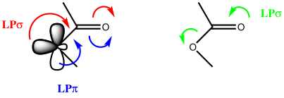
The analysis is based on trying to understand how the components of an ester interact with each other, and in particular how the alkyl oxygen interacts with the carbonyl group. Three electronic interactions in particular can be focused on (below). The first two of these weaken the C=O bond; the last strengthens it. So which effect wins out?

s-cis-ester1

  1. The donation of an in-plane σ lone pair (Lpσ) on the alkyl oxygen into the C=O σ* acceptor (red arrows) 
  2. The donation of an out-of-plane π lone pair (Lpπ) into the C=O π* acceptor (blue arrows)
  3. The donation of an in-plane σ lone pair (Lpσ) on the acyl oxygen into the C-O σ* acceptor (green arrows) 

I will start with computational models, which have the advantage that one can dissect how the vibrations arise. The first two rows show a comparison of the experimental gas phase values[3] with a standard “medium level” ωB97XD/6-311G(d,p) calculation. The discrepancy amounts to ~100-114 cm-1

The carbonyl stretch in esters and ketones
Method: Ester Ketone
Expt (gas phase)[3] 1761 1737
Harmonic ωB97XD/6-311G(d,p) 1860 1851
Anharmonic ωB97XD/6-311G(d,p) 1832 1828
Harmonic ωB97XD/aug-cc-pvQZ 1836 1831
Harmonic CCSD(T)/6-311G(d,p) 1826 1792
Corrected CCSD(T)/6-311G(d,p) ~1774 ~1749
Expt (gas phase) 1761 1737
Reduced CCSD(T)/6-311G(d,p) 1764 1743

There are several possible causes for such errors:

  1. The calculation is for harmonic frequencies; whereas those measured are anharmonic. 
  2. DFT-level force constants at modestly sized basis set levels are known to be too large compared with a complete basis set calculation (CBS). It used to be the practice in fact to routinely scale the force constants down by ~10% to correct for this effect.
  3. The correlation treatment in a DFT approach is incomplete (an error which may in fact be also absorbed into the 10% correction noted above).

So to really get to the root of why an observed ester carbonyl stretch is higher than that of the equivalent ketone, we have to get a handle on these effects above. 

  1. One can calculate cubic and quartic force constants to get an estimate of the effect of anharmonicity on the (harmonic/quadratic) values, which emerges as 23-28 cm-1 
  2. Upping the level of the basis set to aug-cc-pVQZ (close to, but not quite a CBS) reveals further corrections of 20-24 cm-1 
  3. Replacing the DFT method with a CCSD(T)-level treatment of the dynamic correlation gives corrections of 34 and 59 cm-1 respectively for ester and ketone. Assuming the corrections can be treated additively, one can apply the first two to the third, producing “corrected” CCSD(T)/6-311G(d,p) values which are only about 12-13 cm-1 higher than the observed value. This remaining discrepancy is probably due to the difference between aug-cc-pvQZ and a complete basis set (CBS) and any remaining errors in the correlation modelled by CCSD(T). We can be assured now that our theory is reproducing experiment very well.

Now that we can assess the accuracy of our computational methods, we need to try to relate the results to the C=O bond itself. Does turning a ketone into an ester really make it stronger? To directly compare the C=O bond of two different molecules, we need to eliminate the effects of mixing the C=O normal stretching mode with similar energy modes arising from other parts of the molecule. A simple way of estimating this is to set the mass of all but two of the atoms to a very small value (0.00001), leaving only the masses of the C and O as normal; this is shown as a reduced frequency in the table above. The harmonic CCSD(T)/6-311G(d,p) C=O “pure” mode reduces to 1764 for methyl ethanoate and 1743 cm-1 for propanone. So after all of this, at least we now know that the force constant for the C=O stretch really is stronger for an ester. The green arrows seem to win out over the blue/red ones.

One calculation too many? The (Wiberg) bond order for the C=O bond can be derived from the wavefunctions. Its value is 1.635 for ester, and 1.681 for ketone (CCSD/6-311G(d,p)) or 1.766/1.848 (ωB97XD/aug-cc-pvQZ). This is the opposite to that inferred from the carbonyl stretch, and hence favours the blue/red arrows over the green arrows. I set out in this post to try to bring clarity to how an adjacent oxygen influences how we think of the properties of the C=O functional group, but as happens quite often, the answer you get depends on the measurement you make.


‡ The solution values in e.g. acetonitrile are reduced by ~20 cm-1, reaching the values often quoted in text books for these functional groups. † The effect on C-H values is greater, e.g. a reduction from 3186 to 2967 cm-1.

References

  1. W.W. Coblentz, "Infra-red Absorption Spectra: I. Gases", Physical Review (Series I), vol. 20, pp. 273-291, 1905. https://doi.org/10.1103/physrevseriesi.20.273
  2. J.L. Arbour, H.S. Rzepa, J. Contreras‐García, L.A. Adrio, E.M. Barreiro, and K.K.(. Hii, "Silver‐Catalysed Enantioselective Addition of OH and NH Bonds to Allenes: A New Model for Stereoselectivity Based on Noncovalent Interactions", Chemistry – A European Journal, vol. 18, pp. 11317-11324, 2012. https://doi.org/10.1002/chem.201200547
  3. M.W. Wong, K.B. Wiberg, and M. Frisch, "Hartree–Fock second derivatives and electric field properties in a solvent reaction field: Theory and application", The Journal of Chemical Physics, vol. 95, pp. 8991-8998, 1991. https://doi.org/10.1063/1.461230

A golden age for (computational) spectroscopy.

Monday, April 2nd, 2012

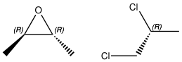
I mentioned in my last post an unjustly neglected paper from that golden age of 1951-1953 by Kirkwood and co. They had shown that Fischer’s famous guess for the absolute configurations of organic chiral molecules was correct. The two molecules used to infer this are shown below.


Using the theory Kirkwood had developed, the prediction for the optical rotation at the sodium D line for the (R,R) enantiomer of epoxybutene (Kirkwood did not use this R,R notation, which was still in the future) was +43°. The measured value was [α]D +59°. The (R,R) enantiomer did indeed correspond to Fischer notation.

QED.

A postscript is that a modern equivalent of Kirkwood’s result, using the ωB97XD/6-311+G(d,p) method gives +67° for the gas phase and +57° for solution (in CCl4). The experimental value relates to the pure liquid. In fact, Kirkwood had been very aware that solvation can influence the measured value of an optical rotation, and so even today, a match between experiment and calculation of ± 16 ° is considered a good fit.

But when it comes to the second molecule, (R)-1,2-dichloropropane, we are in a different ball park. In fact, most of Kirkwood’s article is devoted to unravelling this second system. This is because it was realised that it is conformationally flexible. Two conformations (this term was then often used interchangeably with configuration, which might confuse a modern audience) called trans and skew (now called anti and gauche) were considered and it was realised that the relative populations would be influenced by temperature and particularly, the solvent. I quote here the final conclusion: We have assigned the absolute configuration of Fig. 2 to the dextrorotatory isomer of 1,2-dichloropropane. This was done without any experimental data concerning the optically active forms of the molecule, using only the calculated dependence of the rotatory power on conformation (Table II) and the information about the potential of internal conformation obtained from the electron diffraction and dipole moment measurements.

Non trivial then! Perhaps this is why these techniques were not immediately picked up by synthetic chemists to verify the absolute configuration of their own molecules. But my point is that the use of such techniques now seems to be growing exponentially, which is why this post is headed the golden age of computational spectroscopy. So what of such a modern take on  (R)-1,2-dichloropropane (in heptane, which corresponds to the measured value of +20 to +30, and -21° for the (S) enantiomer). Well, there are in fact three viable conformations, not two as Kirkwood supposed. He did not know that the gauche stereoelectronic effect favoured two of them despite the greater steric encumbrance. The calculated rotations are +53 (anti), +96 (gauche) and -182° (second gauche conformer). Such dependence on conformation is sadly not unusual, and it means you have to know the Boltzmann population very accurately indeed to infer an observed value. This might in part explain the rather circuitous argument used by  Kirkwood for dichloropropane!

Fortunately, nowadays optical rotation (more accurately referred to as optical rotatory power, or ORP) is just one of a growing armoury of spectroscopic measurements that can be computed to the accuracy required to draw firm conclusions. These include ORD (optical rotatory dispersion, or variation with the frequency of the polarised light used), ECD (electronic circular dichroism) and VCD (vibrational circular dichroism). It is still not absolutely routine, but these techniques are now found in an increasing number of synthetic chemists’ toolkits.

And my final reflection is to ponder that the golden age of pharmaceutical synthesis (lets say  1950 – 2000, but  I know I may get dissent), in which certainty about the separate physiological effects of both enantiomers of chiral drugs became mandatory, would not have been possible without Kirkwood’s pioneering article, along of course with Bijvoet’s independent result.

Confirming the Fischer convention as a structurally correct representation of absolute configuration.

Tuesday, March 13th, 2012

I wrote in an earlier post how Pauling’s  Nobel prize-winning suggestion in February 1951 of an (left-handed) α-helical structure for proteins was based on the wrong absolute configuration of the amino acids (hence his helix should really have been the right-handed enantiomer). This was most famously established a few months later by Bijvoet’s definitive crystallographic determination of the absolute configuration of rubidium tartrate, published on August 18th, 1951 (there is no received date, but a preliminary communication of this result was made in April 1950). Well, a colleague (thanks Chris!) just wandered into my office and he drew my attention to an article by John Kirkwood (DOI: 10.1063/1.1700491) published in April 1952, but received July 20, 1951, carrying the assertion “The Fischer convention is confirmed as a structurally correct representation of absolute configuration“, and based on the two compounds 2,3-epoxybutane and 1,2-dichloropropane. Neither Bijvoet nor Kirkwood seem aware of the other’s work, which was based on crystallography for the first, and quantum computation for the second. Over the years, the first result has become the more famous, perhaps because Bijvoet’s result was mentioned early on by Watson and Crick in their own very famous 1953 publication of the helical structure of DNA. They do not mention Kirkwood’s result. Had they not been familiar with Bijvoet’s result, their helix too might have turned out a left-handed one!

I record all this because I was today asked to provide an abstract for an NSCCS Themed Workshop shortly to be held at Imperial College on the uses of the Gaussian computational chemistry program in synthetic chemistry. One of the themes will be chiroptical spectroscopy. Gaussian of course deploys much of the theory developed by Kirkwood in the 1950s to make exactly the same sort of predictions that Kirkwood himself used to verify the Fischer convention in 1951. Whilst the majority of modern determinations of absolute configuration are still based on Bijvoet’smethod, catching rapidly up are those based on chiroptical calculations. Perhaps in 2012 they are trusted more than they were in the 1950s? At any rate, such calculations are nowadays very much part of a modern undergraduate laboratory experience (slightly less so still in research laboratories I fear).

Here is another coincidence. Both Pauling and Kirkwood worked in the same department (Institute of Technology, Pasadena, California). One can only speculate on whether Kirkwood might have wandered into Pauling’s office in late 1951 to alert him that the protein helix should be right rather than left-handed (oh to have been a fly on Pauling’s blackboard). So alerted, would Pauling have foreseen that eventually such determinations would be routinely made using the very quantum mechanics that he had popularised?

Secrets of a university tutor: tetrahedral intermediates.

Sunday, January 8th, 2012

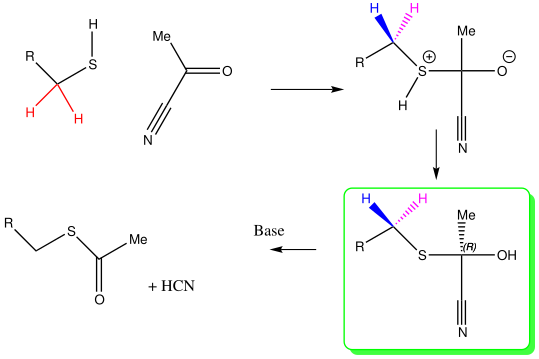
The tetrahedral intermediate is one of those iconic species on which the foundation of reaction mechanism in organic chemistry is built. It refers to a (normally undetected and hence merely inferred) species formed initially when a nucleophilic reagent attacks a carbonyl compound. Its importance to understanding the activity of enzymes cannot be overstated. An example of this genre is shown below, in which a thiol reacts with an acyl cyanide to form the species ringed in green.

The lifetime of such a species is normally assumed to be too short for it to be detectable[1], but suitable adjustment of the substituents enables its lifetime can be extended to many hours. Thus the reaction between PhCH2SH (benzyl thiol) and acetyl cyanide occurs slowly and the resulting intermediate is stable enough to be detected by 1H NMR spectroscopy[2]. The spectrum in CDCl3 is shown below:

Spectrum of a tetrahedral intermediate.

What is shown is actually a difference spectrum, in which the spectrum measured immediately after mixing the two reagents is subtracted from that obtained after about 12 hours. The negative peaks represent a species which is being replaced by one giving rise to positive peaks. It is the nature of these latter peaks which directly prove that the species formed after 12 hours contains an asymmetric tetrahedral carbon atom.

  1. The negative peaks are ~δ1.8ppm (triplet), 3.8 (doublet [assigned to the CH2SH region], 2.6 ppm (the Me group of the acetyl cyanide) and 7.3 (the Ph group).
  2. The positive peaks are 1.9 ppm (Me singlet), an AB quartet at 4.2 ppm equal in integration to the negative peak at 3.8 ppm, and a more disperse Ph peak.
  3. If pressure is applied[3] to the solution, the tetrahedral intermediate forms more quickly, and actually crystallises out of solution (Le Chatelier’s principle).
  4. If a hydroxylamine (RNHOH) is used instead of a thiol, the tetrahedral intermediate forms much more quickly[1], and both N: and O: nucleophilic isomers can be detected[1] (by 15N-13C 2J couplings in the case of the former).
  5. Particularly significant is that the new product manifests its CH2 group as an AB quartet. This must mean that the two methylene protons are diastereotopic (have different chemical shifts and hence the coupling between them can be observed). This cannot be achieved by restricted rotation (atropisomerism) and hence can only arise by the CH2 group being close to an asymmetric (chiral) carbon atom bearing four different groups.
The other interesting aspect is whether the tetrahedral intermediate is formed in two stages, the first being S-C bond formation, followed by a proton transfer from S to O, or whether it can form directly in a single concerted step. On the assumption that CDCl3 solutions contain traces of water, a synchronous mechanism does seem possible. The water helps transfer the hydrogen from S to O, as shown in the intrinsic reaction coordinate[4] animation below (wB97XD/6-311G(d,p)/SCRF=choroform calculation). Notice how the H firstly leaves the S and hops across to the water, and only then does another H from the water hop over to the carbonyl group. The computed free energy barrier for this process is 22.5 kcal/mol, which is pretty much spot on for a slow thermal reaction.

IRC animation for the formation of a tetrahedral intermediate.

The slow motion capture of a tetrahedral intermediate using substituents finely tuned for the purpose (a relatively non nucleophilic thiol coupled with a relatively poor cyano leaving group) enables us to directly prove its identity using NMR. The same technique as it happens was also used to characterise another iconic intermediate, the carbocation, many years after it too was inferred as a key mechanistic participant.

References

  1. A.M. Lobo, M.M. Marques, S. Prabhakar, and H.S. Rzepa, "Tetrahedral intermediates formed by nitrogen and oxygen attack of aromatic hydroxylamines on acetyl cyanide", The Journal of Organic Chemistry, vol. 52, pp. 2925-2927, 1987. https://doi.org/10.1021/jo00389a050
  2. H.S. Rzepa, A.M. Lobo, M.M. Marques, and S. Prabhakar, "Characterizing a tetrahedral intermediate in an acyl transfer reaction: An undergraduate 1H NMR demonstration", Journal of Chemical Education, vol. 64, pp. 725, 1987. https://doi.org/10.1021/ed064p725
  3. N.S. Isaacs, H.S. Rzepa, R.N. Sheppard, A.M. Lobo, S. Prabhakar, and A.E. Merbach, "Volumes of reaction for the formation of some analogues of tetrahedral intermediates", Journal of the Chemical Society, Perkin Transactions 2, pp. 1477, 1987. https://doi.org/10.1039/p29870001477
  4. "C4H9NO2S", 2012. http://hdl.handle.net/10042/to-11696

A lab in a backpack

Friday, April 3rd, 2009

We recently developed a new computational chemistry practical laboratory here at Imperial College. I gave a talk about it at the recent ACS meeting in Salt Lake City. If you want to see the details of the lab, do go here. The talk itself contains further links and examples. Perhaps here I can quote only the final remark, namely that computational chemistry can now provide chemical accuracy for many problems, including spectroscopy and mechanism, and that the basic tools for doing it can easily be carried around in a backpack! Or, perhaps in the not to distant future, an iPhone!