Posts Tagged ‘Imperial College’

Blasts from the past and present: altmetrics.

Sunday, October 13th, 2013

I reminisced about the wonderfully naive but exciting Web-period of 1993-1994. This introduced the server-log analysis to us for the first time, and hits-on-a-web-page. One of our first attempts at crowd-sourcing and analysis was to run an electronic conference in heterocyclic chemistry and to look at how the attendees visited the individual posters and presentations by analysing the server logs.

all_accesses

You can read all about that analysis here. This is one interesting graphic below, showing the 24-hour distribution of accesses. Remember, this was before Google and its analytics even existed (and yes, we were also doing Google-like searches before they did).

hourly-accesses

But let me get to the actual point of this post. A decade or so ago, all universities in the UK were asked to undertake a quality review exercise of their research outputs. One of the metrics of such outputs is the scientific publication, and each research group leader had to collect their most important four articles published in the previous few years and submit them (as paper) to a review panel. This poor panel was faced with a mountain of paperwork (literally!) when they arrived to do their job. It was soon decided that a better (electronic) system had to be devised. So now we have a product called Symplectic (which as it happens originated in the physics department here at Imperial College), which tirelessly gathers such outputs. More accurately, it gathers the meta-data for research publications, since most publishers do not allow actual reprints to be so harvested! And when it finds a new article, it informs its author, and asks them to check that the meta-data is accurate.

So it was a few days ago that I received such an alert. I checked the meta-data (adding in fact some which associates the scientific work with a particular resource, our High-Performance-Computing unit, and also the NMR systems here) but then the following thumbnail caught my eye. The wonderful Symplectic system had computed this for me. 

altmetrics3

This I had to see. Expanded, it shows as follows. An altmetric measures  attention. And attention (however transient) is apparently itself measured by tweets, facebook, news outlets, science blogs, Mendeley and CiteULike

altmetrics1

Well, things have certainly moved on from the days of analysing server-logs! Now, would an aspiring tenure-track young scientist, presenting an altmetric score of 28 to their head of department expect to get their tenure on this basis? Of course, we are back to the old hoary chestnut. Is attention necessarily good? You cannot tell from the above if we have indeed produced worthy science, or science to be scorned.

Well, the above represents a 20 year period in the evolution of science and how it is communicated. Whether this represents positive progress I leave you to decide. And if one of your altmetric scores is > 28, you have done better than us!


Does the icon look familiar? See here.

Computers 1967-2013: a personal perspective. Part 5. Network bandwidth.

Wednesday, June 5th, 2013

In a time of change, we often do not notice that Δ = ∫δ. Here I am thinking of network bandwidth, and my personal experience of it over a 46 year period.

I first encountered bandwidth in 1967 (although it was not called that then). I was writing Algol code to compute the value of π, using paper tape to send the code to the computer. Unfortunately, the paper tape punch was about 10 km from that computer. The round trip (by van) took about a week, the outcome being often merely to discover that the first line of the code contained a compilation error. I think I got to computing π after about six weeks. That is a bandwidth of about 18 characters (108 bits) in 3628800 seconds, or 0.00003 bits per second.

I did my undergraduate work in 1969, when the distance between the card punch and the computer had reduced to about 50m, and instant turnaround involved circulating in a loop between the punch and the line printer, hoping that neither suffered a paper-wreck. The bandwidth had certainly gone up. On a good day, you could make 20 or so circuits, which did leave one feeling faintly dizzy. 

The next improvement came in 1972, when I was solving non-linear equations for kinetic rate constants, using a 110 bits per second (baud) or ~ 18 characters per second using the 6-bit computers of that era) teletypewriter. This was about 50m from the lab where the kinetic measurements were made (using, if you are interested a scintillation counter. Yes, I was mildly radioactive for most of my PhD, but I do not believe I glowed in the dark). This bandwidth was in fact fine for uploading kinetic data, and receiving the computed rate constant and its standard error. You might note however that this teletypewriter was the only one in the building I occupied, and yet demand for it was small (I was pretty much its only user). 

The next increment occurred in Texas 1974-1977, where I was now doing quantum chemical calculations. Back in time to the card punch and the lineprinter (Texas is big, and so now the distance between them was a 10 minute walk). But in my last year there, a state-of-the-art 300 baud teletypewriter was installed! This was now fast enough to play a computer game (something to do with Dragons and Dungeons I think), and so now there was competition to use it. Particularly from one of my friends, who shall be called George, and who on one occasion spent about 48 virtually contiguous hours trying to get to the last level. The rest of us returned to the card punch to submit the calculations. It was also during this period that the first emails started to be exchanged, but only really as a curiosity: “it would never catch on” was the opinion of most.

Back in the UK by 1977, I was overwhelmed by the speed of the 9.6 kbaud graphics terminal I now had access to, 32 times faster. And the rate continued to multiply, by a further 1000 to attain 10 Mbaud in 1987. But another change occurred during this period. The previous eras had involved transmitting the data no more than ~200m, from one point in the campus to another. But by 1986, if one tried hard enough, one could reach ARPANET. And that was 5000 km away! My first use of such distances was to reach California and download Apple’s system 5.0 for the Macs in the department (I have described elsewhere the role the Mac’s printer port played in this). From then on, we always did have the latest operating system installed on most of the machines (although not always did this subterfuge address the intended issue, which was to stop the computer crashing as often).

These speeds however did not reach beyond the university. Back home, around 1983, I was back to using a 300 baud modem, with an acoustic coupler to the land line. Our young daughter, aged 3 at the time, joined in the data transmission with gusto. Her joyful shrieks were invariably picked up by the acoustic coupler, and translated into a jumble of characters, which were then interleaved into the numbers coming back from quantum calculations. It was sometimes difficult to tell them apart! These domestic modems gradually got faster, probably attaining 9.6 kbaud by about 1993 (during the course of which the acoustic component was replaced by electronics, and oddly, our daughter stopped shrieking in quite the same way). 

Back in the university in 1993, the first 100 megabits per second (100Mbps ≅100 Mbaud) ethernet lines and switches were being installed, but the national and international backbones were still a lot slower. It was in this year that I was approached to be part of a SuperJanet project. We were going to do a molecular videoconference from London to Cambridge and Leeds; a three-way connection, and this needed ~ 20Mbps to transmit the signal from the video camera as well as the 3D images of molecules in real-time (compression techniques were not so advanced in those days). Because BT was sponsoring the project, they naturally wanted some publicity, and so we even got to appear on the national television news that night. But we came within about 1 minute of a disaster. Our 20Mbps connection went through the SuperJanet national backbone, the capacity of which was, you guessed, ~ 20 Mbps. The network operators (located at the Rutherford-Appleton laboratories), who we had not had the foresight to pre-warn, came within 1 minute of isolating Imperial College from the national network because of our bandwidth hogging. I met them a month or so later, and they told me this. I feel I was lucky to escape with my life and body intact from that meeting (or to put it another way, they were not happy bunnies). 

By about 2000, I had achieved 1 Gbps to my desktop computer (and there it has stayed for the past 13 years). What about home? Well, to cut the story short, I recently benchmarked the domestic WiFi connection between a laptop and “the world” at about 65 Mbps (download) and 18 Mbps (upload), a little less than 1 million times greater than 30 years earlier and a 12 orders of magnitude greater than in 1967. I gather however that some lucky inhabitants of Austin Texas (the scene of my 1974-1977 experiments), courtesy of Google, can get 1 Gbps!

I will end by quoting Samuel Butler, writing in 1863I venture to suggest that … the general development of the human race to be well and effectually completed when all men, in all places, without any loss of time, at a low rate of charge, are cognizant through their senses, of all that they desire to be cognizant of in all other places. … This is the grand annihilation of time and place which we are all striving for, and which in one small part we have been permitted to see actually realised” (Quoted in George Dyson, “Darwin amongst the Machines, The Evolution of Global Intelligence”, Addison-Wesley, N.Y., 1997. ISBN 0-201-400649-7).


I just benchmarked my office computer (using only solid-state memory and that 1Gbps connection) and got 58Mbps (download)/75Mbps (upload).

The standard program was NCSA Telnet if  I remember. You made a connection from the computer (using its printer port) to the ARPANET node at University College London (not a widely advertised service), and thence to an Apple FTP site where one could initiate an anonymous file transfer back to one’s computer.  System 5 was about half a Mbyte then, and this took about 1-2 hours to retrieve (unless the connection went down, in which case one started again).

Digital repositories. An update.

Saturday, July 21st, 2012

I blogged about this two years ago and thought a brief update might be in order now. To support the discussions here, I often perform calculations, and most of these are then deposited into a DSpace digital repository, along with metadata. Anyone wishing to have the full details of any calculation can retrieve these from the repository. Now in 2012, such repositories are more important than ever. 

In the UK, the main funding organisations are increasingly requiring researchers to deposit their primary data in such open archives, and some disciplines are better than others at this (chemistry does not rank very highly in general however in terms of deposition of data). Our DSpace server is a local one running at Imperial College, but a few months back I became aware of Figshare, which aspires to operate on a much wider and more general scale.  So I have injected one of the calculations reported in another post (the IRC for the sodium tolyl thiolate reaction with dichlorobutenone) into Figshare, making use of the API which has recently been developed for this purpose and implemented by  Matt Harvey. As with DSspace, it issues a DOI, which can be then quoted wherever appropriate (and particularly in scientific articles). This particular deposition is 10.6084/m9.figshare.93096

This repository is still undergoing a lot of development, but already one can see many interesting features, such as export to Endnote or Mendeley, and a QR barcode for devices with cameras. I would encourage anyone who regularly generates e.g. computational chemistry data, or knows a group that does, to encourage them to make use of such facilities.

Postscript: If you have a look at this deposition in Figshare you may already notice some of the developments I note above.  Matt Harvey (who, with Mark Hahnel of Figshare, developed our publish script) has added to the entry:

* A data descriptor document URL

* Wikipedia and pubchem links (automatically resolved from Inchi/Key searches)

* Links to chemspider searches

* Links to all other objects in the  Spectra DSpace repository with a common Inchi/Key

Confirming the Fischer convention as a structurally correct representation of absolute configuration.

Tuesday, March 13th, 2012

I wrote in an earlier post how Pauling’s  Nobel prize-winning suggestion in February 1951 of an (left-handed) α-helical structure for proteins was based on the wrong absolute configuration of the amino acids (hence his helix should really have been the right-handed enantiomer). This was most famously established a few months later by Bijvoet’s definitive crystallographic determination of the absolute configuration of rubidium tartrate, published on August 18th, 1951 (there is no received date, but a preliminary communication of this result was made in April 1950). Well, a colleague (thanks Chris!) just wandered into my office and he drew my attention to an article by John Kirkwood (DOI: 10.1063/1.1700491) published in April 1952, but received July 20, 1951, carrying the assertion “The Fischer convention is confirmed as a structurally correct representation of absolute configuration“, and based on the two compounds 2,3-epoxybutane and 1,2-dichloropropane. Neither Bijvoet nor Kirkwood seem aware of the other’s work, which was based on crystallography for the first, and quantum computation for the second. Over the years, the first result has become the more famous, perhaps because Bijvoet’s result was mentioned early on by Watson and Crick in their own very famous 1953 publication of the helical structure of DNA. They do not mention Kirkwood’s result. Had they not been familiar with Bijvoet’s result, their helix too might have turned out a left-handed one!

I record all this because I was today asked to provide an abstract for an NSCCS Themed Workshop shortly to be held at Imperial College on the uses of the Gaussian computational chemistry program in synthetic chemistry. One of the themes will be chiroptical spectroscopy. Gaussian of course deploys much of the theory developed by Kirkwood in the 1950s to make exactly the same sort of predictions that Kirkwood himself used to verify the Fischer convention in 1951. Whilst the majority of modern determinations of absolute configuration are still based on Bijvoet’smethod, catching rapidly up are those based on chiroptical calculations. Perhaps in 2012 they are trusted more than they were in the 1950s? At any rate, such calculations are nowadays very much part of a modern undergraduate laboratory experience (slightly less so still in research laboratories I fear).

Here is another coincidence. Both Pauling and Kirkwood worked in the same department (Institute of Technology, Pasadena, California). One can only speculate on whether Kirkwood might have wandered into Pauling’s office in late 1951 to alert him that the protein helix should be right rather than left-handed (oh to have been a fly on Pauling’s blackboard). So alerted, would Pauling have foreseen that eventually such determinations would be routinely made using the very quantum mechanics that he had popularised?

The dawn of organic reaction mechanism: the prequel.

Sunday, November 13th, 2011

Following on from Armstrong’s almost electronic theory of chemistry in 1887-1890, and Beckmann’s radical idea around the same time that molecules undergoing transformations might do so via a reaction mechanism involving unseen intermediates (in his case, a transient enol of a ketone) I here describe how these concepts underwent further evolution in the early 1920s. My focus is on Edith Hilda Usherwood, who was then a PhD student at Imperial College working under the supervision of Martha Whitely.1

The doctoral degree itself had only been introduced into British universities in 1919,1 and so Usherwood was very much a forerunner of the modern system of training.The academic staff and students at Imperial totalled 30, making it one of the largest research schools in UK chemistry at the time. Usherwood’s project was on tautomers, or isomers of molecules which differ only in the position of a labile hydrogen atom. The then quite novel electron-pair symbolism introduced by G. N. Lewis’ in 1916 was adopted to represent two tautomeric equilibria (the supposed mobile or tautomeric hydrogens being enclosed in […])2

  1. [H]C:::N ⇔ C::N[H]
  2. [H]C:::CH ⇔ C::CH[H]

or in our more modern representation (in which lines replace colons, and charges are used to ensure the octet rule is adhered to when possible):

  1. H-C≡N ⇔ C≡N+-H
  2. HC≡CH ⇔ :C=CH2

Modern structural techniques such as electron diffraction or microwave spectroscopies not yet existing, the problem was tackled using specific heat measurements as a function of temperature. This method suggested to Usherwood that for e.g. equilibrium 2, the concentration of iso-acetylene (we now call this vinylidene) was insignificant at ordinary temperatures, but it became appreciable between 200-300°C. Further evidence was claimed for the formation of the “unseen” vinylidene by observing ketene as a by-product of the oxidation of acetylene. This article very much set the trend of (an almost mandatory) speculation on the outcome of (nowadays much more complex) reactions by the need to formulate a reaction mechanism in which various (otherwise undetected but) plausible intermediates are involved.

Moving on some 90 years, and how might one approach such a problem nowadays? Well, I have oft argued on this blog that a good place to obtain an immediate reality check on a proposed mechanism is a calculation. It will come as no surprise that a very accurate calculation can be done on the systems shown above. For example, CCSD(T)/cc-pVTZ will yield a free energy for the equilibria with a pretty small error (< 1 kcal/mol). We use ΔG = -RT Ln K to inter-convert free energies and equilibrium constants. If we are generous and state that in order to observe an appreciable concentration of a minor species, the equilibrium constant can be no smaller than 10-3, its energy cannot be greater than 4 kcal/mol above the more abundant isomer. Our reality check will be to see if the free energy of vinylidene is indeed no more than 4 kcal/mol greater than acetylene. Well, CCSD(T)/cc-pVTZ predicts vinylidene is 41.3 kcal/mol higher @298K, reduced to 33.8 @2000K (and before you ask, these results took a total of perhaps 30 minutes to obtain).

In 1924, the concept of calculating the relative energies of two species using first principles was not even a glimmer on the horizon. The nature of mechanisms was slowly and often painfully established by recourse to experiments alone. And many of the unseen intermediates often remained just such, their existence only inferred indirectly from the models one constructed (of specify heats in Usherwood’s case). It is perhaps no great surprise that these models do not always stand the test of time. In this case, within a year of Usherwood’s publication, Partington was suggesting that the model for the specific heats of acetylene should have included allowance for polymer formation.3 The modern take, armed with the calculation I note above, might in fact side with Partington after all. As for the formation of ketene by oxidation, it is indeed known that (peracid) oxidation of an alkyne will produce ketene, but the modern mechanism (an interesting exercise in arrow pushing for a student) does not involve vinylidene intermediates.

I will add at this point that Hilda Usherwood was married to Christopher Ingold, and the pair of them subsequently published many of the seminal articles in what became known as physical organic chemistry. That legacy continues to this day with (as I noted above) the almost mandatory speculation about the mechanism of any new reaction. But it is only in the last five years or so that these speculations have started to be increasingly tested against reliably accurate computation. A new era is underway.


1 My post was inspired by reading W. H. Brock, “The case of the Poisonous Socks”, chapter 28, RSC Publishing, 2011, 978-1-84973-324-3.

2 These representations are taken from ref 1, p 225 (and including a correction of replacing C:C as drawn there by C::C). The original article apparently appeared in the proceedings of the British Association of 1924, which is not yet available online.

3 Brock, in ref 1, p226, suggests that Usherwood stood her ground on this one, and won her case by showing that Partington’s evidence for polymerization was valid for only a small part of the temperature range she had investigated. I have not managed to track down the original sources for this exchange.

Henry Armstrong: almost an electronic theory of chemistry!

Monday, November 7th, 2011

Henry Armstrong studied at the Royal College of Chemistry from 1865-7 and spent his subsequent career as an organic chemist at the Central College of the Imperial college of Science and technology until he retired in 1912. He spent the rest of his long life railing against the state of modern chemistry, saving much of his vitriol against (inter alia) the absurdity of ions, electronic theory in chemistry, quantum mechanics and nuclear bombardment in physics. He snarled at Robinson’s and Ingold’s new invention (ca 1926-1930) of electronic arrow pushing with the put down “bent arrows never hit their marks“.1  He was dismissed as an “old fogy, stuck in a time warp about 1894.”1 So why on earth would I want to write about him? Read on…

He did worthy (nowadays this could mean dull) chemistry on e.g. naphthalenes, but I want to focus on two articles from the period 1887-1890 (10.1039/CT8875100258  and 10.1039/PL8900600095). Let me set the scene by reminding of an earlier post showing the structure of a bis(stilbyl)ketone, dated 1921. The two aromatic groups (yes, they really are such) are drawn in the manner we would nowadays draw cyclohexane. This practice in fact continued in texts and articles for perhaps 30 more years! Not much sign of electronic accounting there then! And by a professor at Imperial College no less, where Armstrong had been.

Aromatic molecule, circa 1921

So when would you date the diagrams below? So called Clarrepresentations, originating from the 1950s? The one on the bottom below cites Clar and dates from 2010, DOI: 10.3390/sym2031653, but the one above it comes from Armstrong’s 1890 article!

Two representations of pyrene, 2010 and 1890.

Clar representations are used to count electrons (as coming in six packs). But there is little doubt that Armstrong’s use of a “C” (or inner circle, which is exactly what it is) means six as well. The evidence I present below, taken from his 1887 article.

Armstrongs six pack

  1. He counts the six carbons as having a total of 24 what he calls affinities (definition: An attraction or force between particles that causes them to combine), or four per carbon. Let us make life easy and equate affinity=electron (remember, the electron itself was not yet discovered or named!). He disposes of 12 affinities/electrons to form what we now call six carbon-carbon σ bonds, and a further six for the  six C-H bonds.
  2. He is left with exactly six affinities/electrons, which he presupposes to act upon each other, in the manner of resultants (the old term for vectors). In fact, he replaces these six vectors by a circle (the inner circle) in his second article of 1890.
  3. He invents delocalization in all but name when he states that any one atom has an influence on other atoms not contiguous to it in the ring (he really did have o/m/p directing influence in mind here).
  4. He compares the introduction of a substituent (R, which comes from the old name Radicle) perturbing the distribution of the affinity to how electric charges perturb each other. So, the affinity behaves as if it might have electrical (from which the name electron came of course) properties? And it might be described by a vector?
  5. Remember, this is a scientist who in later life did not believe in electronic theories of chemistry? Really? Well, again in 1890:

Is this an affinity (=electronic) theory of chemistry?

  1. Here, he is refining his vector representation of affinities, saying that these vectors in effect define a circle, an inner circle no less. One that can be disrupted  (Robinson some 30 years later wrote of how the cycle of six electrons are able to form a group that resists disruption) when an additive compound is formed (his examples are all electrophiles, what we now call electrophilic addition) such that the remaining carbons become merely unsaturated. There seems little doubt he is describing what we now call a Wheland Intermediate.
  2. Is this really a man who did not believe in electronic theories of chemistry? What about that concluding paragraph then? The laws of substitution require a knowledge of the inner structure of (what we now call the aromatic) hydrocarbons?
  3. And that such speculations may suggest fresh lines of experimental inquiry? This all sounds very much like the modern use of quantum mechanics and its electronic eigenvectors to describe the probability distribution of electrons (remember, Armstrong did not approve of this either) to probe the inner structure of molecules and to suggest new experiments.

We have a real mystery. Armstrong got so very close to a modern theory of chemistry. Was he asleep when Stoney named the electron around 1891 and Thomson discovered it in 1897? If only he had followed his own advice! Ah well, just as well he was ignored in the 20th century when he preached against it all.


  1. W. H. Brock, “The case of the Poisonous Socks”, chapter 20, RSC Publishing, 2011, 978-1-84973-324-3
  2. Clar, E. The Aromatic Sextet; Wiley: New York, NY, USA, 1972.

Computers 1967-2011: a personal perspective. Part 1. 1967-1985.

Thursday, July 7th, 2011

Computers and I go back a while (44 years to be precise), and it struck me (with some horror) that I have been around them for ~62% of the modern computing era (Babbage notwithstanding, ~1940 is normally taken as the start of the modern computing era). So indulge me whilst I record this perspective from the viewpoint of the computers I have used over this 62% of the computing era.

  1. 1967: I encountered (but that term has to be qualified) my first computer, suggested to me as an alternative to running quarter marathons on Wimbledon common at school by an obviously enlightened teacher! I wrote a program (in Algol) on paper tape, put the tape in an envelope, and sent it off to Imperial College (by van) to run, on an IBM 7094. A week later, printed output showed you had made a mistake on line 1 of the program. As I recollect, after about eight weeks of this, I got the program to run (and calculated π to 5 decimal places).
  2. 1970: By now I was a student (again at Imperial College), and was introduced to Fortran, then a radical new innovation to a chemistry degree. The delightfully named pufft compiler combined with the 7094 again, but this time with punched Holerith cards as input and line printer output. I cannot remember what we were asked to program. I do remember that the punched cards were produced by a pool of punch card operators, working from code pages written by the programmer. Some students (not me!) thought it great fun to give their Fortran variables naughty names (which the punch card operators then refused to punch, thus causing the student to fail the course!).
  3. 1971: I really liked this programming lark, so when instant-turnaround was introduced that year, I decided to do a proper program. It was called NLADAD (yes, I was no good at names, even then), which stood for non-linear-analysis of donor-acceptor complexes. The idea was to take recorded NMR chemical shifts, and fit them to an equilibrium A+B ⇔ AB+B ⇔ AB2 using non-linear regression analysis. It must have been all of 200 lines of code (OK, I did not write the matrix inversion routine myself)! Instant turnaround was also great, you got to punch your own cards this time, and had the great excitement of feeding them into a card reader yourself. You then walked about 5 yards to the line printer and waited agog. No waiting one week, this was less than a minute. Or it would have been if the line printer did not paper-wreck every two minutes! (I might add that I have a dim recollection of a member of the computer centre staff standing by to recover these paper wrecks. He, by the way, is now the director of the ICT division here!).
  4. 1972: I am now doing a PhD (yes, boringly, yet again at Imperial College). I had found the one and only teletypewriter in the chemistry department. The crystallographers had secreted it away in their empire, but were very dismayed to find me occupying it constantly. Instant was now even more instant. I was now connecting to a time-sharing CDC 6400 computer, at the dazzling speed of 110 baud (or bytes per second). These were small bytes by the way, since the CDC used 6 bits per byte. The result was that one did everything in UPPER CASE, since a 6-bit byte only allows 64 characters! My (still Fortran) programs reached probably 1000 lines of code now, and I was engrossed in deriving non-linear analyses of steady state chemical kinetics (about four different kinds of rate equation as I recollect). Ah, the joys of covariance analysis, and propagation of errors (I was in a kinetics lab, and all the other students plotted graphs on graph paper, and if pressed, plotted gradients of graphs, the so-called Guggenheim plots. I thought this the dark ages, but no-one volunteered to join me in this single teletypewriter room. Not even the attractive girls in the group. I was the geek of my time, no doubt about that. My kinetic analysis did however have one upside. Its how I meet my wife to be a few years later!).
  5. 1974: PhD completed, I was now ready to go to Texas, where everything is bigger (and in terms of computers, slightly better, a CDC 6600 now and a 300 baud teletypewriter!). I had been computing now for seven years, and finally I actually got to SEE the device for the very first time. My mentor, Michael Dewar, had a sort of special relationship with the university. His students (and possibly only his students) were allowed to go into the depths of the machine room, where behind plate glass you could see the CDC 6600. I soon learnt how to get even closer. It was not particularly exciting however. I was more entranced with the CALCOMP flatbed plotter, which was located next to the 6600. Pictures at last (you probably do not want to know that to convert my kinetics in 4 above to pictures, I got quite expert in using a french curve. Look it up before you jump to conclusions). Part of the pact I negotiated was that I was only allowed into the inner sanctum at 03:00 in the morning (sic!). Still a geek then! Oddly, I was one of the few students in Dewar’s group using the CALCOMP, but at least we now had pictures of the molecules I was now calculating (using MINDO/3). To put the computing power into context, in 1975, Paul Weiner, another group member, announced that he had completed a full geometry optimisation of LSD, this having taken about 4 days to do on that over-worked 6600. The entire group went out to celebrate. Many pitchers of beer were drunk that nite.

    Computer graphics from 1976.

  6. 1977: Back to Imperial, where we might have also now had a CDC 6600. And a Tektronix terminal running at the dizzying (hardwired end-to-end) speed of 9600 baud. I learnt to Word process on this device (using a word processor, written in Fortran, although not by me) and I wrote three review articles by this means, using a fancy phototypesetter as the printer. My next program, STEK, probably ran to about 5000 lines of code, and it persuaded the Tektronix to plot all sorts of things, ball&stick diagrams, isometric potential surfaces, molecular orbitals, and the like (and jumping ahead, my experience with this program eventually led to CML, and Peter Murray-Rust, but that is indeed jumping ahead). I think I also managed to gain access to the Imperial machine room, that inner sanctum, yet again. But for reasons I will not go into, it was not as interesting as the Texan machine room.

    Chemistry Computer graphics, circa 1977-85.

  7. 1979: I encountered a Cray 1 computer, and probably also 8-bit bytes (and yes, lower case printer outputs) for the first time at the University of London Computing Centre.
  8. 1980: Remember that teletypewriter, encountered earlier. Well these were now running at 2400 baud and I started to organise the deployment of a chemistry department computer network to sprinkle several such terminals around the department. The controller was a PAD, and in that year, we introduced STN ONLINE using this network. It was the first time we could search CAS online ourselves (previously, it was a service offered by the library). Literature searching has not been the same since.
  9. 1980: I finally again encountered a real computer, which one could happily listen to without creeping into machine rooms in the middle of the night. It was the data system on a Bruker Spectrospin 250 MHz superconducting NMR spectrometer. I had many adventures on this system. It was installed, by the way, on more or less the same day as the birth of my first daughter Joana. It had a hard drive (5 Mbytes as I recollect, and cost an absolute fortune, around £10,000 if I remember correctly).

    Combining Quantum mechanics and NMR.

    Computer graphics 1982, from NMR spectrometer.

  10. 1982: More networks, this time a curious computer known as the Corvus Concept, using a networked hard drive (possibly as big as 20 Mbytes by now), and a large screen.
  11. 1985: Enter the Mac (OK, the IBM PC came a little earlier, but it was not entrancing). Now one really had a tactile computer that made noises (not always nice), produced smoke signals occasionally, and ejected its floppy disk incessantly. Yet another revolution to cope with. As I type this, I look down on that Mac, which is still underneath my desk. Wonder if its worth anything on ebay?

Well, a second consecutive blog, with (almost) no pictures or molecules. And I have only gotten to the half way stage of my story. Better break off then.

What is the future of books?

Friday, April 29th, 2011

At a recent conference, I talked about what books might look like in the near future, with the focus on mobile devices such as the iPad. I ended by asserting that it is a very exciting time to be an aspiring book author, with one’s hands on (what matters), the content. Ways of expressing that content are currently undergoing an explosion of new metaphors, and we might even expect some of them to succeed! But content is king, as they say.

Here I list only some innovative solutions which have emerged in the last year or so, but which also raise important issues which we ignore at our peril.

  1. TouchPress were one of the first publishers to get off the mark with their living books. Their first offering was The Elements, deriving from an earlier interactive display of the periodic table (an example of which can be seen in the entrance to the chemistry building at Imperial College). It is a programmed book, in the sense that the content is expressed using code written by the publisher (very much in the manner of interactive games).
  2. Next to appear were Inkling, who describe their offering as interactive. Their approach is described in a blog written by their founder, Matt Macinnis. There he talks about The Art of Content Engineering, which again makes it sound as if authoring a book is in effect programming it! (I know what he means; if you follow the link to the talk I allude to above, you may spot that it too is, at least in part, programmed, and not simply written). Inkling also promote the book as part of a social network, with readers able to annotate the content, and share that annotation with others.
  3. The latest company to change the way books are both read and authored is Pushpoppress, the heart of which is also an interactive app.
  4. Then there is the epub3 format. This is a free and open standard for e-books. This third revision in particular is meant to enhance interactivity.

Something of a common theme so far. Books are going to be interactive! But what about these issues?

  1. Each of the first three (commercial) publishers above has adopted their own programming format. Although HTML5 may be at the heart of some of this, programming may also mean control (in the sense that the creative industries must put control of their content at the heart of what they do). Each of the first three above sound like a closed system, and extracting re-usable content is, I argue, an essential part of doing science. I am just a tad worried that the approaches exemplified above may not allow this to happen.
  2. Suppose you manage to acquire a chemistry textbook in any of the four approaches listed above. Will they inter-operate, in the sense of being able to extract data from one and perhaps inject it into another? Or will each be a data- or information silo, rigidly controlled by the creative content generator (whoever that is)?
  3. What might an aspiring author, intent on creating interactive content do? Should they go closed/proprietary or open? They will clearly need to retrain themselves. We have indeed come a long way along the road: hand-written manuscript → typed manuscript → word-processed manuscript → interactive app! Like computer games, is the day of the single-authored book rapidly fading, to be replaced by a large team, each with their own tasks to perform?

I end with this question. Is the era of books, just like the Web itself, going to be the app? And who will be able to (find the time) to participate?

Monastral: the colour of blue

Tuesday, March 8th, 2011

The story of Monastral is not about a character in the Magic flute, but is a classic of chemical serendipity, collaboration between industry and university, theoretical influence, and of much else. Fortunately, much of that story is actually recorded on film (itself a unique archive dating from 1933 and being one of the  very first colour films in existence!). Patrick Linstead, a young chemist then (he eventually rose to become rector of Imperial College) tells the story himself here. It is well worth watching, if only for its innocent social commentary on the English class system (and an attitude to laboratory safety that should not be copied nowadays). Here I will comment only on its colour and its aromaticity.

Copper phthalocyanine

In 1933, Hückel was still thinking about his molecular orbital electronic theory of benzene, but for ~15 years, there remained little need for the rule we now know as 4n+2, because n was invariably equal to 1 for most known aromatic molecules! It was only the discovery of so-called non-benzenoid aromatics in the 1940s (e.g. Dewar’s tropolone structure) that propelled chemists to identify aromatic molecules with other values of n. And Monastral blue is a prime example of n=4 (although it would be of interest to find out when it became so associated with the Hückel rule). If you count the red bonds above, there are eight, along with one lone pair of electrons located on the highlighted (blue) nitrogen atom. This makes 18 π-electrons in the ring, or 4×4+2 (there are paths other than the one shown, but they give the same count). Part of the reason for the remarkable thermal stability of this molecule must be its aromaticity.

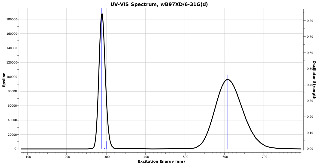
So what about the colour? The visible spectrum is shown below, with λmax ~ 610 and 710nm.

Visible absorption spectrum of copper phthalocyanine.

Well, a TD-DFT ωB97Xd/6-31G(d) calculation reveals the following. This reproduces the band at 610nm very nicely, but leaves the identity of the band at  710nm mysterious. How does that originate? One might speculate that this could arise from the presence of another species. Thus copper phthalocyanine itself is neutral, but it could easily be oxidised to a cation, and this could then form a  1:1 π-complex with a second molecule of the neutral radical (DOI:10.1021/ja00238a021 )

The electronic excitation at ~610nm arises from the following MOs:

Orbital 147, the highest occupied MO (HOMO). Click for 3D

Orbital 148, the lowest unoccupied MO.

The unpaired electron in copper phthalocyanine occupies the following rather interesting orbital, which appears not to be involved in its blue colour.

Orbital 146. The singly occupied MO.

So, just as with mauveine, a mystery remains. The colour of Monastral blue is not monochromatic, in that it appears to be caused by two bands in the 600-700 region. Calculation however reveals it to have only one band at 610nm. What is the other one?

The colour of purple

Thursday, February 24th, 2011

One of my chemical heroes is William Perkin, who in 1856 famously (and accidentally) made the dye mauveine as an 18 year old whilst a student of August von Hofmann, the founder of the Royal College of Chemistry (at what is now  Imperial College London). Perkin went on to found the British synthetic dyestuffs and perfumeries industries. The photo below shows Charles Rees, who was for many years the Hofmann professor of organic chemistry at the very same institute as Perkin and Hofmann himself, wearing his mauveine tie. A colleague, who is about to give a talk on mauveine, asked if I knew why it was, well so very mauve. It is a tad bright for today’s tastes!

Charles Rees, wearing a bow tie dyed with (Perkin original) mauveine and holding a journal named after Perkin.

The first thing to note about mauveine is that it is not a single compound; actual samples can contain up to 13 different forms! These all vary in the number of methyl groups present which range from none up to four, in various positions. These compounds all have absorption maxima λmax in the range 540-550nm, the colour of purple. The structure of one of these, known as mauveine A, is shown below.

Mauveine A. Click to load 3D

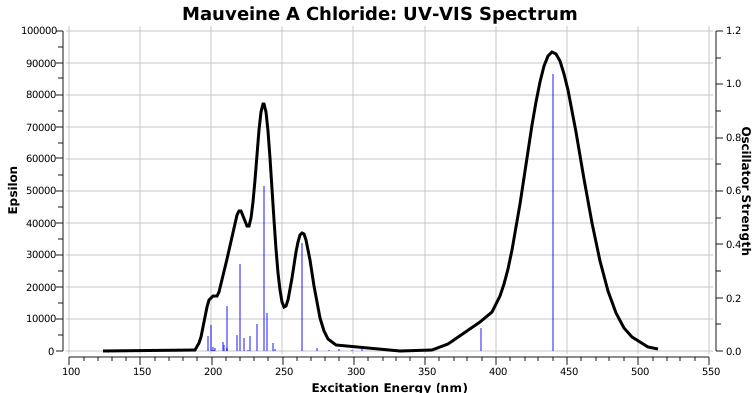
You can see from this that something is missing. The so-called chromophore is a cation, and an anion needs to be provided to balance the charge. We will now attempt to predict the color of purple using purely the power of quantum mechanics (for many years, accurate prediction of colour was a holy grail amongst dye chemists for obvious reasons). The anion can be chloride, and the colour is often measured in methanol as solvent. So the first task is to calculate this ion-pair. This used to be easier said than done (and in the past, the anion was often simply neglected). But using the ωB97XD density functional procedure (to get the van der Waals interactions modelled correctly) and a 6-311++G(d,p) basis set, coupled with a smoothed-cavity continuum solvation procedure, and two molecules of water (standing in for methanol, which is a bit bigger) as explicit solvent molecules, we get the structure apparent when you click on the diagram above (DOI: 10042/to-7320). Application of time-dependent density function theory (TD-DFT) gives a measure of the UV-optical spectrum (below, loaded as a scaleable SVG image. If you are using a modern browser, it should display. If not, try the latest FireFox, Chrome, Safari etc).


This has several noteworthy aspects.

  1. The visible (right hand side) part of the spectrum is very monochromatic, with λmax ~440nm. In other words, mauveine has a pure and intense colour.
  2. This λmax is hardly affected by the presence of the counterion.
  3. The electronic transition responsible for this band is a simple HOMO (highest-occupied-molecular-orbital) to LUMO (lowest-unoccupied-molecular-orbital) excitation of an electron.
  4. These orbitals are shown below.
    LUMO HOMO

    Mauveine A. LUMO. Click for 3D

    Mauveine A. HOMO. Click for 3D

  5. Note how the excitation involves the central region of the molecule, and one of the pendant aryl groups, but not the other. One might presume that tuning the colour would only work if changes are made to the first of these aryl groups.
  6. There is a real mystery about the calculated value of λmax, which differs from the observed value by about 100nm (the wrong colour, making mauveine orange rather than purple). Normally, this sort of time dependent density functional theory has errors no greater than 15-20nm. The calculated value of λmax is not sensitive to the basis set, or the presence or not of the counter ion and solvent. Clearly, a discrepancy of this magnitude must have some other explanation. Watch this space!

So this post ends with a bit of a mystery. The fanciest most modern computational theory gets the colour of mauveine wrong by ~100nm. Why?